Simulated Evolution
An implementation by
John R. Nash
This MS-DOS based program demonstrates the concept of simple evolution by an iterative
process involving reproduction, mutation and natural selection, all
in an interactive graphical environment that let’s you control
the simulation in real time. It is an example of an automated system
attempting to solve a problem by trial and error, making minor
adjustment towards an “optimal” solution, a solution not
always not always predicted of by the programs author. With
MS-Windows it will run in full screen DOS mode.
The program does not fit neatly into any established category since
it requires NO interaction to use so it is not a game although
most people find it very entertaining (and almost hypnotic) even if
they are not interested in the underlying scientific concepts.
At the same time it is a serious educational tool for teaching the
concepts of computer evolution.
The program randomly pre-populates the simulation screen with a few bugs (white squares)
and a certain amount of bacteria (green dots). See screen shot
below. Each bug has six “genes” which control how they
move. When a bug bumps into bacteria, it eats it and gains energy.
This is good for the bug as each move a bug makes uses a small amount
of energy so if a bug doesn’t eat enough bacteria it will die.
Once a bug is mature and if it has enough energy, it will reproduce
by splitting into two new bugs, each inheriting the genes from its
parents but with a twist. The genes will be slightly mutated so the
offspring will have slightly different movement patterns than the
parent. This mutation, spread out over many generations can lead to
distinct species, which have movement patterns optimized for their
environment. As the simulation progresses you will see the bugs
color change to indicate their health and status as follows: White:
Normal, Blue: High energy, Red: Low Energy, Magenta: Imminent
reproduction: Cyan: Almost strong enough to reproduce but reaching
end of life (rare condition).
Download and Installation
Download Program and Source Code:
There are temporary links until files are uploaded to SourceForge.net
Download Simulation Evolution Program
here. (480KB)
Download Simulation Evolution Source Code
here. (70KB) Contribute to the
sev.SourceForge.net project!
To run, unzip/decompress into a directory and run the SE.EXE file. No installation is required but the file EGAVGA.BGI,
which is the graphics driver, must be in the same directory. A
number of other files are included such as pre-defined simulations
and source code for the program for those with an interest.
Once started the program will immediately begin the simulation after displaying
the credits. The simulation window will appear (shown below)
and contains bugs (white squares), bacteria (green dots), population
graph, menu and simulation statistics. At the start, and throughout
the simulations, bacteria are deposited randomly on the screen at a
constant rate. The simulation window is the universe in which the
bugs and bacteria are contained. It is a “closed universe”
which means that if a bug reaches the edge of the simulation window
it will reappear at the other side of the simulation window headed in
the same direction. In terms of topology the bugs and bacteria live
on the surface of a sphere.
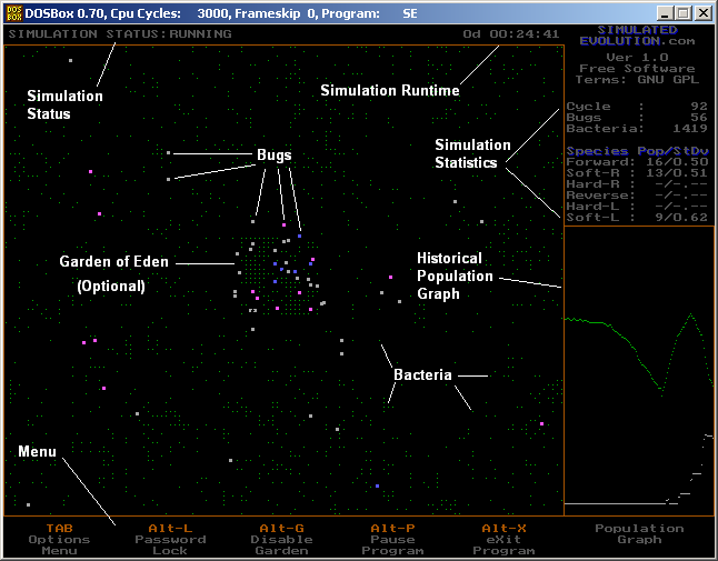
Displayed In the upper right hand corner, under the program credits is the Cycle
counter and the population counts for both bugs and bacteria. The
Cycle counter is incremented every 800 bug moves and closely tracks
the number of generations elapsed.
The bugs survive by searching out and feeding on bacteria. Their movement patterns
dictate their success. As a local area becomes depleted of bacteria
a bug must either move to a non-depleted area of bacteria or starve.
Each bug has six genes, the value of which dictates the probability
of moving in that direction. The six directions are Forward,
Right, Hard Right, Reverse, Hard Left and Left.

When the simulation is started ten bugs are placed on the screen with genes very close to
equal. This means that each bug has an almost equal chance of moving
in any given direction and therefore appears to “jitter”
in one place. Since their local bacteria are quickly depleted
some turn red and die. A minimum number of 3 bugs are artificially
kept alive so as to keep the simulation running if necessary. Bugs
who survive to the age of 800 moves and have at least 1,000 units of
energy (blue) become mature (magenta) and reproduce by fission. They
divide into two new bugs each with half the energy of the parent and
slightly mutated genes. A bug’s genes remain unchanged for the
duration of its life. They are either adequate for that bug to gather
enough bacteria to reach maturity, from each of which is derived40
units of energy allowing 40 moves, or inadequate meaning the bug will
either die of starvation (red) or of old age (cyan).
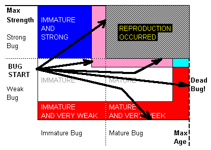
The color of the bugs is significant and is indicative of their age, strength, or both
as follows. After reproduction, the two new bugs will each have 1/2
of the strength of the parent which will cause them to start with a
white color. The life cycle of a bug will end in either reproduction,
or death by starvation or old age as shown below.
The bacteria are the green dots
that are randomly replenished on the screen. The represent food for
the bugs and each one that is eaten gives a bug 40 units of energy
allowing more 40 moves.
The Garden of Eden is an area in the center of the simulation window with a higher
density of bacteria, which is also replenished at a higher rate. The
purpose of the garden is to provide an additional environment that
could potentially foster new species called twirlers. A twirler is a
bug with genes that cause it to “twirl” either counter
clockwise or counter-clockwise, each of which would represent two
distinct species. A twirler would be more likely to stay in the same
general area rather than “trolling” across the screen in
search for new areas of food. Any twirlers that developed which
migrate out of the garden tend to die quickly as they deplete the
food in their local area. Many of the garden attributes can be
controlled though he tab menu to see how different settings change
the simulation dynamic.
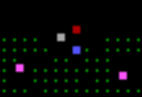
Here is a magnified section of the edge of the garden from the screen shot available in
the Introduction. The bacteria are green while the bugs can be
identified by the color legend (below).
Population Graph
The population graph in the lower right hand corner graphs both bug population (white) and
bacteria population (green). It should be noted that the bacteria
population in the garden (if the garden is enabled) is not displayed
in the graph but is included in the Bacteria count above. The garden
is discussed in further detail in the section Options Menu.
A species as defined by this program is two or more bugs that have a common gene whose
standard deviation falls below a certain threshold. Standard
deviation is a statistical term indicating how “spread out”
the magnitude of a series of numbers is. If the genes were all equal
they would have a very high standard deviation, conversely if one
gene had a high value and the others were all zero, you would say the
genes had a very low standard deviation. The weight of the numbers
would be concentrated in one gene. In this program it would mean
that a bug with a low standard deviation has a tendency to move in a
given direction much more often than any other. It could be any one
of the six genes mentioned above. The top-right section of the
screen, just above the population graph, shows the number of bugs
that match the criteria for classification as a species for each of
the six genes and what their average standard deviation (StDv) is.
The menu along the bottom of the screen shows the Hot-Key options for the main menu.
They include the following options.
<TAB> or <Right-Arrow>
- Replaces the population graph with an options menu that can be navigated with the <TAB> key.
<ALT-L>
- Initiates the screen saver. This locks the screen until the correct password is
entered. If no password is present the user will be prompted for
one. Note: an unregistered copy will first prompt the user for a
bypass key in order to enable this function. If you have not
registered your program then this function is not available.
<ALT-G>
- Toggles the state of the garden. The garden is a rectangular area in the center
of the screen that, when enabled, has a higher density of bacteria
than the rest of the screen. If a bug developed genes that allowed
it to stay in the garden and take advantage of the plentiful food
supply then it would flourish. This is basically a variation in the
bugs environment that allows for more species to develop. Note:
Just because the garden is enabled does not necessarily mean that
other species will develop, it is purely a matter of chance.
<ALT-P>
- Paused the simulation until a key is pressed.
<ALT-X> or <ALT-Q>
- Ends the simulation and exits the program. Note: the simulation is NOT
saved.
-

After the <TAB> key is pressed and the options menu appears the selected option will
be bordered by a yellow rectangle. The <TAB> key will move the
rectangle to the next field or the <Right-Arrow> key will move
to the top of the next menu. As a menu option is highlighted the
Hot-Key options bellow the simulation window will be updated and a
brief description of the option will be displayed at the extreme
bottom right of the screen. The available options with their
defaults and function are as follows.
Change Password
- Allows the user to change the password. This is the password the user must enter in
order to bypass the password lock or screen saver. If one exists
then the user will be prompted for old password before being allowed
to change it. Note: an unregistered copy will first prompt the user
for a bypass key in order to enable this function. If you have not
registered your program then this function is not available.
Change Garden Width [50 - 85]
- Option: Gard Width
- Default: 70
- Allows the user to change the width of the garden, if the garden is enabled. Note: the resolution of
bacteria on the screen it such that a change in the width of less
than four may not visibly change the size of the garden. A larger
garden is more likely to allow the evolution of new species and
would also be able to support a higher population.
Change Garden Height [50 - 85]
- Option: Gard Hight
- Default: 70
- Allows the user to change the height of the garden, if the garden is enabled. Note: the resolution of
bacteria on the screen it such that a change in the width of less
than four may not visibly change the size of the garden. A larger
garden is more likely to allow the evolution of new species and
would also be able to support a higher population.
Change Bacteria Screen Rate [1 - 40]
- Option: S Rate
- Default: 4
- The rate bacteria are deposited on
the screen. Value represents number of bacteria deposited on screen
every turn. A turn being each time every bug moves once. A higher
rate allows more bugs to survive and changes the simulation
dynamics.
Change Bacteria Garden Rate [1 - 20]
- Option: G Rate
- Default: 8
- The rate bacteria are deposited on
the garden, if the garden is enabled. Value represents number of
bacteria deposited on bacteria every turn. If Garden has maximum
number of bacteria already then no bacteria are deposited. A higher
rate allows more bugs to survive and changes the simulation
dynamics.
Allow Mutation of Maximum Bug Age [T/F]
- Option: M Age
- Default: F
- Enables (T) or disables (F) the
mutation of the maximum age a bug can achieve. This could
conceivably allow a species of bugs with longer or shorter lifespan
to evolve but it is unlikely unless a different lifespan is somehow
a survival trait. The logging file would have to be consulted to see
if this had actually happened. UNTESTED.
Allow Mutation of Maximum Bug Strength [T/F]
- Option: M Str
- Default: F
- Enables (T) or disables (F) the
mutation of the maximum strength a bug can achieve. This could
conceivably allow a species of bugs with a higher or lower maximum
strength to evolve but it is unlikely unless it would somehow
translate into a survival trait. The logging file would have to be
consulted to see if this had actually happened. UNTESTED.
Allow Mutation of Bug Maturity [T/F]
- Option: M Mature
- Default: F
- Enables (T) or disables (F) the
mutation of the age at which a bug becomes mature. This could allow
a species of bugs that becomes mature at a lower age to evolve. The
logging file would have to be consulted to see if this had actually
happened. UNTESTED.
Allow Mutation of Minimum Reproduction Strength [T/F]
- Option: M ReproStr
- Default: F
- Enables (T) or disables (F) the
mutation of the strength required for reproduction (maturity). This
could allow a species of bugs that reaches maturity at a lower level
of strength UNTESTED.
Allow Mutation of # of Genes involved in a Mutation [T/F]
- Option: Severity(B)
- Default: F
- Specifies the number of variables mutated on a scale of 1-255 with 255 indicating a maximum of 6
variables. A value of 43 is just about one sixth of the maximum and
therefore causes one gene to be mutated for each new bug UNTESTED.
Allow Mutation of Mutation Severity[T/F]
- Option: Severity(G)
- Default: F
- Specifies the mutation severity, on
a scale of 1-255 for each variable mutated with 255 indicating a
maximum change of 6. A value of 43 is just about one sixth of the
maximum and therefore causes each mutated gene to increase or
decrease by only one UNTESTED.
Save Simulation to ASCI File [<filename>]
- Option: Save Simulation
- Saves the current simulation to the
file specified by the user. The user is only allowed to specify a
filename; the extension of .SIM is automatically assigned. The file
created is a user modifiable text file and can be edited with
certain restrictions. See the section on Saving/Loading Simulation
Files for more information.
Load Simulation from ASCI File [<filename>]
- Option: Load Simulation
- Loads the simulation file specified
by the user. The user is only allowed to specify a filename; the
extension of .SIM is automatically assigned. As with the command
line parameters, if the file exists, the current simulation is saved
to TEMP.$$$ and the new simulation loaded with the defaults of the
specified file. If the file does not exist a warning is issued and
the previous simulation is resumed.
Protect Garden from Vertically Moving Bugs [T/F]
- Option: Protect Garden
- Default: T
- Enables (T) or disables (F) protection of the garden species from the species of vertically
moving bugs. During early testing it was discovered that species
that evolved in the garden had a high probability of being wiped out
by forward moving bugs that chanced upon the trick of moving
vertically through the middle of the screen, thus allowing them to
steal food from the garden more often then a forward moving bug
would otherwise. Code was added to randomly change the direction of
a vertically moving bug that was headed toward the garden. Early
testers said this was unfair as I was artificially modifying the
environment but I countered that this problem would not exist in a
sufficiently large simulation grid and that I was compensating for
the limited simulation space. To solve the argument this option was
added allowing the user to enabled this feature as desired. Note:
This phenomenon is a perfect example of the bugs in the program
taking advantage of a food source, or a characteristic in their
environment, un-conceived of by the author.
Enable Logging [<filename>]
- Option: Logging
- Default: F
- Allows the user to enable (T) or disable (F) logging. When logging is enabled the user is prompted
for a new filename (an extension of .LOG is assumed). After
correctly entering and confirming a filename the file is created and
logging begins if file did not previously exist, otherwise logging
information is appended to the existing file. In either case
simulation statistics are logged to the file until is exceeds the
maximum size specified by “M File Size” (below). See
the section on Logging for more information.
Set Logging Period [1 - 65536]
- Option: Log Period
- Default: 10
- Specifies the interval, in seconds,
to update the *.LOG file if logging is enabled. Range is from 1
second to 65536 seconds. See the section on Logging for more
information.
Set Maximum Log Size [1 - 500]
- Option: M File Size
- Default: 1 (100K)
- Specifies the maximum size in 100’s
of KiloBytes that the logging file can grow to. Range is from 1
(100 kilobytes) to 50 (5 Megabytes). If the Log Period (above) was
set to 1 second then the maximum value would allow over 8 hours of
log history before shutting logging off. If the user wanted to
graph a simulation longer than 8.6 hours then reduce the log period.
Set Timer for Simulation Auto-Termination [0 - 65536]
- Option: Min To Run
- Default: 0
- Allows the user to specify a time limit that the simulation is to run in minutes.
Range is 0 - 65536 minutes. Zero value causes simulation to run
forever. Even longer times can be specified by editing and loading a
simulation file. See Saving/Loading Simulation Files for more
information. This function is useful when running multiple
simulations from a DOS batch file. See section on Automating
Simulation Series for more information.
Logging is an option for those users who need to know more about a simulation than what is
shown in the simulation window and the population graph. It also
provides a sometimes-surprising glimpse into the dynamics of the
evolution of one or more species.
Then logging is enabled the user is prompted for a new filename (an extension of .LOG is assumed). After
correctly entering and confirming a filename the file is created and
logging begins if file did not previously exist, otherwise logging
information is appended to the existing file. In either case
simulation statistics are logged to the tab delimited file until is
exceeds the maximum size specified by “M File Size”
(above). If a simulation file and logging file are specified from
the command line but logging is disabled in the *.SIM file the fact
that logging was specified in the command line will override the
simulation file and logging will be enabled to the specified log
file.
The log data is stored in a standard CSV format that can be easily imported into your
favorite spreadsheet or database program. To do so for MS-Excel for
example, first import the *.LOG file as a space delimited file. Once
in a standard spreadsheet format you would arrange all columns
desired to be graphed so they were adjacent. Then select the
appropriate column headers and all the fields in the columns you wish
to graph. Then click on graph button, draw a rectangle with the
crosshairs that the mouse cursor becomes and answer all questions
appropriately. For more detailed instructions consult the user
manual for your spreadsheet or database software.
You will probably want to make separate graphs for the species population and the
species Standard Deviation. These two usually give an interesting
perspective of the simulation
If file previously existed then a header is first appended showing when logging started.
Then the column header is added as shown in the example below. The
file is then updated with all applicable fields at the rate
determined by the “Log Period” until logging is stopped,
the program is halted, or the size of the log file reaches the
maximum file size as specified by “M File Size”.
All fields are delimited by one or more spaces and are defined as follows…
|
Column |
Description |
|
D |
# of days simulation has run |
|
Time
|
Hours:Minutes:Seconds simulation has run |
|
C |
# of cycles elapsed |
|
Pop |
# of bugs currently on screen |
|
BactS |
# of bacteria on Screen (not including garden) |
|
BacG |
# of bacteria in Garden |
|
P0..5 |
Population of each of the 5 possible species |
|
SD0..5 |
Average Standard Deviation for each of the 5 possible species |
|
MStr |
Average Maximum Strength of all bugs |
|
Mage |
Average Maximum Age of all bugs |
|
Repr |
Average Reproduction Strength of all bugs |
|
MRSt |
Average Age of Maturity of all bugs |
|
MS |
Mutation Severity (G) - as defined in the menu |
|
MB |
Mutation Severity (B) - as defined in the menu |
|
GH |
Garden Height |
|
GW |
Garden Width |
|
SL |
# of bacteria placed on screen per turn |
|
GL |
# of bacteria placed in garden per turn |
|
P |
Whether garden protection is enabled (0 or 1) |
As an example of how log file analysis can provide a more detailed look
into the simulation dynamics, here are two graphs of a basic
simulation using default parameters and no Garden of Eden.
The first graph (below) shows the relative population of the Bacteria
vs. the Bugs for the first 89 cycles, prior to the development of
any distinct “species”. For clarity, the population
values of the bugs and the bacteria are shown relative to the
maximum population of each so that they are presented on a common
scale, similar to that of the the simulation graph. As no species
exist prior to cycle 89, there is no standard deviation value to
graph.
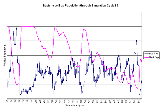
In the first graph (above) you can see that the Bug population
oscillates in a somewhat erratic fashion but is generally out of
sync with the bacteria population sine when more bugs are present
they are consuming bacteria at a faster rate which causes the
bacteria population to fall. When the bacteria population falls too
far it is insufficient to support the bug population and the
vulnerable bugs begin to die off, allowing the bacteria population
to increase only to start the cycle over again.
The second graph (below) shows the relative population of the Bacteria
vs. the Bugs starting at the point where a population of forward
moving bugs first evolves (cycle 90) and is detectable via the
standard deviation threshold of the program. As in the first graph,
the population values of the bugs and the bacteria are shown
relative to the maximum population of each.
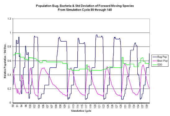
In the second graph (above) you can see that with the evolution of a
distinct forward moving species, the Bug population oscillates in a
much more distinct fashion and is clearly 180 degrees out of phase
with the Bacteria population. During the period graphed the bugs
have stumbled on the optimal movement pattern (forward movement) to take advantage of
the simulation environment and any other changes in the genes are
due primarily to random mutation rather than environmental
pressures.
Saving and Loading Simulation Files
Simulation files store all aspects of a simulation so a simulation can be saved and continued
at a later time. The simulation file is stored in a ASCII text file,
allowing the user to modify it with almost any text editor in order
to tailor a simulation to their liking. For information on the
format and editing of simulation files see the sub-section
Custom
Simulation Sets.
If a simulation file is specified the program checks to see if it exists. If the
simulation file is found then it is loaded and the simulation
proceeds using that saved simulation as a starting point. If the
specified simulation file is not found then an error message is
displayed and a new simulation is started with the default settings.
Trying to load an invalid simulation file will most likely result in
a runtime error, or at the very least, undesirable results.
It is assumed that the <simulation-file> has an extension of .SIM and that the
<log-file> has an extension of .LOG so they do not need to be
included in the command line. If filenames with different extensions
are included they are removed and replaced with either .SIM or .LOG.
Example. “SE TEST.TXT FUN.CAP” would attempt to load
simulation file TEST.SIM and start logging to FUN.LOG.
If the user wants to restore a simulation prior to an unsuccessful load, the running
simulation is saved to a file named TEMP.$$$ each time a simulation
is loaded for just such a reason. Rename it to TEMP.SIM and then
load it with SE TEMP.
Advanced Operation and Automation
Options for running the program in a MS-DOS
With Window XP, you cannot natively run 16 bit MS-DOS programs in a window so this
program will only run in full screen mode. The program will actually
run best in full screen mode as it will be very fast and give you the
best visual experience. Even so, some people may want to run the
program other Windows based Operating System platforms or in a window
on a MS-Windows XP which I actually had to do in order to take
advantage of the Windows screen shot utilities.

For that, I use, and recommend, a program called
DOSBox
7.0 which is, in effect, a x286 DOS emulator with full EGA,VGA support.
As it is software based emulator there is a significant performance
penalty but some of the advantages include the fact that you can
minimize the program and the simulation will continue to run. After
installation and obtaining a emulated DOS window, you must mount your
local drive so that you can access your files. For example, to mount
my local C:\ drive I used the command “
Z:>
mount c c:\<your-sub-directory>”.
Great for testing or running multiple simulations at the same time.
This program will accept up to two command line parameters in the following format
SE <simulation-file> <log-file>
The program assumes that the <simulation-file> has an extension of .SIM and that
the <log-file> has an extension of .LOG so they do not need to
be included in the command line. If filenames with different
extensions are included they are removed and replaced with either
.SIM or .LOG. Example. Each of the following would attempt to load
simulation file TEST.SIM and log to RUN1.LOG (“SE
TEST.SIM RUN1.LOG” = “SE TEST.TXT RUN1.TXT” = “SE
TEST RUN1”). See the section on Saving/Loading
Simulation file for more information.
If the log file is found then logging is activated and logging information is appended
to the existing file. If the log file is not found then it is
created. In either case simulation statistics are logged to the file
until is exceeds the maximum size specified in the Options Menu. See
the section on Logging for more information. Note that the Log file
size in in 100KBytes, NOT MegaBytes!
Seeded (Canned) Simulation Sets
Executing the SE.EXE program with no parameters will create a new simulation with 10 bugs,
each with randomized genes and position. You may want to start with
the same exact simulation if you are doing some experimentation with
the settings and comparing the results for multiple simulations. The
following .SIM files are provided with the identified attributes.
Feel free to modify them or add your own to the collection. If you
do re-distribute simulation files, please include some explanation
about their intended purpose.
SET_00.SIM
- This file is a sample default simulation with no modifications except that the
garden is turned off to begin with. It is provided as an example
only. It contains the same settings that you might get if you
started the program without specifying a simulation file (except
that the garden is of) and is provided as a reference only.
SET_01.SIM
- This file is the same as SET_00.SIM except that the first bug has enhanced genes
such that it contains has a strong tendency to move forward. In
addition, the screen environment has been modified such that the
Density of bacteria in the Screen has been doubled as shown in the
line below:
- 4.0000000000E-03 rSLIMPCT
- The first letter ‘r’ indicates a Real number, the ‘S’
indicates Screen, the ‘LIM’ indicates Limit and the
‘PCT’ indicates Percent. (see the section Editing
Simulation Files below for more information).
- Using this
simulation file should result in the decedents of the forward moving
taking over the environment as their genes will be more highly
evolved. When running this simulation, the bugs will sometimes die
off (drop to 3 or less) and the system will artificially keep some
alive with random genes. Playing with the Screen Limit, one may be
able to create a more stable simulation.
SET_10.SIM
- This file is a
modification of a simulation that was running for just over 20
minutes with the garden is on. All bugs were removed except for 6.
Each of the 6 bugs has a different one of it’s six genes set
to be dominant (value of 8) and has the forward moving gene set to
slightly influence the movement (value of 1). In the case of the
bug with the dominant forward moving gene, the gene to move to the
right was set to a 1.
- The object of
this simulation is to jump start the evolution process by creating a
viable parent for a species with a predominate gene and seeing how
they fare in the given environment. Setting the non-dominant gene
to 1 causes a ‘rotating’ bug that might otherwise occupy
the exact same space as another with very similar movement patterns
to occasionally shift over and occupy a new space.
SET_11.SIM
- This simulation
is identical to SET_10.SIM (above) except that each of the 6 bugs
does not have a non-dominant gene set to 1 to skew the default
movement.
- The object of
this simulation is almost identical to SET_10.SIM but will
demonstrate the even a ‘pure’ pre-dominant gene will
eventually become somewhat corrupt due to mutation. As each
generation occurs and takes on the mutated genes of it’s
parents, it will develop non-zero values in the other non-dominant
genes that will cause two bugs with the same genes (and therefore
movement patterns) to possibly drift apart.
SET_12.SIM
- This simulation is identical to SET_10.SIM (above) except the Bacteria density of
the garden has been increased and the bacteria density of the screen
has been decreased as follows.
1.2000000000E+00	        rSDENSITY
8.2500000000E+00           	rGDENSITY
5.0000000000E-04           	rSLIMPCT
3.0000000000E-01           	rGLIMPCT
- The object of this simulation is identical to SET_11.SIM but will allow more bugs
and possibly more species to exist in the garden.
SET_13.SIM
- This simulation is identical to SET_11.SIM (above) but with the same bacteria
density modifications in SET_12.SIM
- The object of this simulation is identical to SET_11.SIM but will allow more bugs
and possibly more species to exist in the garden.
Simulation files are stored in a ASCII text file, allowing the user to modify it with
almost any text editor in order to tailor a simulation to their
liking. SE.EXE performs limited error checking when loading a
simulation file so extreme care must be used when modifying a
simulation file.
Guidelines for modifying a simulation file: 1.) Always start with a known good file.
If you are unsure then start a fresh simulation (with no command
line parameters) and save it to a new file. 2.) Never add extra
spaces or carriage returns. Try to retain original formatting of
fields as much as possible. 3.) When changing a value never change
it outside its allowed range. Most fields only require a small
change to observe results in simulation dynamics. 4.) When modifying
a long integer (32 bit word) be aware that fields of this type are
stored in two 16 bit words, one representing the high word and one
representing the low word. 5.) Be aware that the numeric value of
fields stored in the simulation file may differ from the same field
displayed in the user menu. For instance in the user menu the field
Min To Run has a range of 0-65536 and represents minutes; in the
simulation file it has a range of 0 - 4294967296 (of which the high
end would be represented as a high and low word of 65536 65536). In
addition, the value stored in the simulation file is in 10’s of
milliseconds instead of minutes, so a value of 1 entered in the
program and then saved to a simulation file would show up in the
following format: (6000 0). If all of this seems too confusing then
don’t worry about it. Most everything you would ever want to
do with this program can be done through the user interface of the
program. Access to the simulation file is offered to appease the
hard-core enthusiasts that would otherwise feel limited. 6.) If you
get a runtime error or undesirable results then make a less drastic
change to the file and try again.
The basic format of a simulation file along with descriptions of fields, possible ranges
of variables and recommendations as to whether they are user
modifiable follows…
Example Format for Simulation File
[HEADER INFORMATION]

[GLOBAL]

  0 00 00 59         Days, Hours, Mins & Secs 	Don’t Change!
12 0                 Cycle_Cntr, Low Word / High Word	Don’t Change!
32                   NumofBugs			Must match bug quantity (below)
666                  Bact_on_Screen		Don’t Change!
244                  Bact_in_Garden		Don’t Change!
1                    GardenOn			1 or 0
 1.2000000000E+00    rSDENSITY			Keep floating point format
 6.2500000000E+00    rGDENSITY			Keep Floating point format
70                   bGARDWID			50-85
70                   bGARDHIG			50-85
 2.0000000000E-03    rSLIMPCT			Keep Floating point format
 1.7400000000E-01    rGLIMPCT			Keep Floating point format
0                    tMAXAGE			1 or 0
0                    tMAXSTR			1 or 0
0                    tMATURE			1 or 0
0                    tREPROSTR			1 or 0
1                    tGProtect			1 or 0
42                   bMUTRATNG			1-255
42                   bMUTRATMS			1-255
DEFAULT              Log File Name		8 char string
0                    tLogging			0 or 1
1000 0               Log Period in 10s of mSec	Long Integer (Guideline #4)
1                    Max Size of Log file in 100Kb	1-50

0 0    Elapsed time   at which to end program (0=NoEnd)
							Long Integer (Guideline #4)
       Time in 10s of mSec in form of LowWord, HighWord
0 0    Elapsed Cycles at which to end program (0=NoEnd)
							Long Integer (Guideline #4)
       Cycles in form of LowWord, HighWord

# Note that the number of bugs must exactly match the NumofBugs variable above!

[BUG X] (Sample Bug)

578                  age			1-MAXAGE (below)
889                  str			1-MAXSTR (below)
5                    dir			0-5
58                   posx			4-498
401                  posy			22-438
7                    colr			Don’t Change!
1000                 MAXAGE			16-65520
1500                 MAXSTR			16-65520
800                  MATURE			16-65520
1000                 REPROSTR			16-65520
5                    gene[0]			(-100) - 100
1                    gene[1] 			(-100) - 100
-1                   gene[2] 			(-100) - 100
-5                   gene[3] 			(-100) - 100
-2                   gene[4] 			(-100) - 100
2                    gene[5] 			(-100) - 100
[GRAPH CTRL] changing anything below [GRAPH CTRL] risks crashing the program
Automating Multiple Simulations
I was able to automate twelve one hour simulations and send logging to different
log files by performing the following steps. 1.) Starting and saving
a new simulation to S1.SIM; 2.) Editing S1.SIM as desired, i.e.
setting elapsed time to one hour (Low Word 32320, High Word 5) Note
this could been done in the simulation much easier before saving it
to the S1.SIM file; 3.) Creating and executing a batch file as
shown below:
SE S1 L1 (Loads simulation S1.SIM and sends logging to L1.LOG)
SE S1 L2 (Loads simulation S1.SIM and sends logging to L2.LOG)
SE S1 L3 (Loads simulation S1.SIM and sends logging to L3.LOG)
SE S1 L4 (Loads simulation S1.SIM and sends logging to L4.LOG)
Different initial conditions could have been used for each of these simulations by creating different simulation files.
Simulated Evolution is 100% FREE!
So that the maximum number of people may benefit from this program, I am releasing it as
free software, under the terms of the GNU GPL, for anyone to use or
modify as they wish. I hoipe you enjoy using the program as much as I did writing it.
This program is free software: you can redistribute it and/or modify it under the terms of the GNU
General Public License as published by the Free Software Foundation,
either version 3 of the License, or (at your option) any later
version.
This program is distributed in
the hope that it will be useful, but WITHOUT ANY WARRANTY; without
even the implied warranty of MERCHANTABILITY or FITNESS FOR A
PARTICULAR PURPOSE. See the GNU General Public License for more
details.
You should have received a copy of the GNU General Public License along
with this program. If not, see <
http://www.gnu.org/licenses/>.
Visit
http://www.SimulatedEvolution.com for shared simulation files, user group forums and program updates.
Modifying the Program (Source Code)
The source code for this program is provided in the directory “
./source”.
You can download Turbo Pascal 5.5 (or possibly other versions) from Borland’s web site at
http://dn.codegear.com/article/20803.
After installation and setup of Turbo Pascal, you will need to
compile each *.PAS file into a binary TPU file (Turbo Precompiled
Unit file) by loading it, changing your destination to disk (as
opposed to memory) and then pressing F9. Note that the SE_IO.PAS
file was too big to load and was truncated so I have two versions,
one with comments and the other without. The one without comments
seems to load and compile just fine. At some point in the past I was
able to load and compile the larger one so it is probably just a
memory setting in the Turbo Pascal program? If you are going to work
with the source code to add or enhance features why not join the
Simulated Evolution Open Source project on
www.SourceForge.net?
Design Considerations / Programmer Notes
This program was written by John Nash of Scottsdale Arizona. This
particular implementation is based on a similar program first written
by Michael Palmiter, Temple City, CA., as described by the article
“Simulated Evolution: wherein bugs learn to hunt bacteria by
A.K. Dewdney
” in
Scientific American (Computer Recreations), May 1989.
I started this project in 1981. The program is written in Borland
Turbo Pascal 5.5 which is now freely available (ironically, as
“Antique Software”) from Borland here
http://dn.codegear.com/article/20803.
The bugs are stored in a circular double-linked list. The bugs and
bacteria are stored directly in VGA video memory and when a bug
checks for bacteria the program has to access each pixel of video
memory surrounding a bug. This means that the program is video
intensive and its performance will vary depending on the type of bus
your video card is on (i.e. PCI vs. ISA). The advantage to this is
that the user sees everything that happens because it happens in
video memory.
After watching the simulation for any period of time the user will notice that the
simulation seems to speed up when the bug population drops and slow
down when it increases. The reason is that the computer has to do
more work per turn (one turn being the time to move each bug) when
there are more bugs. The bugs of course are oblivious to real time
as long the food is placed on the screen according to bug moves and
not real time.
The user might have also noticed that the graph will speed up or slow down depending on
how fast bug time is moving. This is because the graph is being
updated every 50 bug moves. I tried updating it by real time but the
graph got skewed as the bugs moved faster, the graph rate stayed
constant and the rise of bacteria was much more pronounced than the
fall. The logging file however is updated according to real time.
This might seem like a discrepancy but the logging interval is
usually much longer than the graph update interval so I don’t
think the skew is be statistically significant.
This program was implemented with a language that did not include a library or
framework for a graphical user interface (window-based or otherwise).
As such, all interaction with the user had to be explicitly captured
and processed and if a key sequence was not completed in a timely
manor, generate a timeout and return the simulation to its default
state. This effort strongly reinforced the quantum leap in ease of
programming represented by development tools which handle the
complexity of user interface logic inside the framework (Win32
Software Development Kit (SDK) introduced in 1991) so the programmer
didn’t have to which allows them to concentrate on the
conceptual aspects of the program rather than the tedious aspects of
I/O. Since then, there are many frameworks with even easier
implementation models such as server side scripting languages with
strong support of HTML and XML (PHP, Ruby for Rails & Java for
example). With the larger frameworks and more feature rich user
interfaces comes a performance penalty however so a MS-DOS
implementation, such as this, delivers maximum performance.
Future development goals included a distributed simulation grid such that
bugs leaving the edge of the screen travel over a network (TCP
sockets) and appear on a “virtually adjacent” computer
thereby forming a multi-system simulation grid which can expand the
simulation size and overall performance. As Turbo Pascal 5.5 does
not have a native TCP/IP socket library, this would have required a
re-implementation in later generation language or linking to a 3
rd party library or writing one in assembler.
 Table of Contents |
Download Program |
Blog about this section |
Compile and modify Program |
Open Source Project


 The Garden of Eden is an area in the center of the simulation window with a higher
density of bacteria, which is also replenished at a higher rate. The
purpose of the garden is to provide an additional environment that
could potentially foster new species called twirlers. A twirler is a
bug with genes that cause it to “twirl” either counter
clockwise or counter-clockwise, each of which would represent two
distinct species. A twirler would be more likely to stay in the same
general area rather than “trolling” across the screen in
search for new areas of food. Any twirlers that developed which
migrate out of the garden tend to die quickly as they deplete the
food in their local area. Many of the garden attributes can be
controlled though he tab menu to see how different settings change
the simulation dynamic.
 After the <TAB> key is pressed and the options menu appears the selected option will
be bordered by a yellow rectangle. The <TAB> key will move the
rectangle to the next field or the <Right-Arrow> key will move
to the top of the next menu. As a menu option is highlighted the
Hot-Key options bellow the simulation window will be updated and a
brief description of the option will be displayed at the extreme
bottom right of the screen. The available options with their
defaults and function are as follows.


 For that, I use, and recommend, a program called DOSBox
7.0 which is, in effect, a x286 DOS emulator with full EGA,VGA support.
As it is software based emulator there is a significant performance
penalty but some of the advantages include the fact that you can
minimize the program and the simulation will continue to run. After
installation and obtaining a emulated DOS window, you must mount your
local drive so that you can access your files. For example, to mount
my local C:\ drive I used the command “Z:>
mount c c:\<your-sub-directory>”.
Great for testing or running multiple simulations at the same time.